As, Spark DataFrame becomes de-facto standard for data processing in Spark, it is a good idea to be aware key functions of Spark sql that most of the Data Engineers/Scientists might need to use in their data transformation journey.

callUDF

One of the most vital functions of Spark, which I found useful in my day to day usage. callUDF is used not only to call the user defined functions, but also to utilise the functions of Spark Sql which are not a part of Spark functions objects.

Example:

For example parse_url is a part of Spark Sql but not available in Spark’s functions object. Hence its not possible to use it directly as a part of your DataFrame operations, you need to wrap it in callUDF function.

val df= Seq((“http://spark.apache.org/path?query=1"),("https://people.apache.org/~pwendell/spark-nightly/spark-master-docs/latest/api/sql/#negative")).toDF("url_col")
df.withColumn("host", callUDF("parse_url", $"url_col", lit("HOST")))

Input_file_name

This function is used to get the file name of the current spark task. Mostly used in debugging or to find out the specific files which have bad records.

Example:

df.withColumn(“filename”, input_file_name)

spark_partition_id

To get the specific spark partition id.

df.withColumn(“partition_id”,spark_partition_id)

na

na is Spark DataFrame api function, which is used to drop or fill null values.

Example:

df.na.drop()

will drop all the rows which containing any null values.

df.na.drop(Seq(<cols>))

drop all the rows which contain null values in the specified columns

df.na.fill(“literal”)

Fill the null values with the specified literal

agg

Aggregate function is used to compute different aggregate expressions over different columns.

df.groupBy(“dept”).agg(min(“id”), count(“id”), avg(“salary”))

struct

Struct function is used to create new struct from existing columns.

Example:

One on the most common use case of this functions is to create JSON values from existing columns.

val df1 = Seq(Seq("Arun","Vijay","vinay"),Seq(1,2,3)).toDF("Name","id")
df1.select(struct("*").alias("json"))

transform — DataFrame API

Transform function is used to chain spark transformation functions. This function helps to breaks the big spark transformation queries into modular and chain them later.

Example

val df = Seq(1,2,3).toDF(“id”)
def incByOne(df: DataFrame): DataFrame = {

  df.withColumn("inc", df("id") +1)

}
val incDf = df.transform(incByOne)

Transform — Spark Sql

Spark Sql also posses an transform function to work with array elements.

Example:

To increment one by each element of an array

Spark.sql(“SELECT transform(array(1, 2, 3), x -> x + 1)”)

Both Spark sql transform function and Dataframe Transform function are different and exists for different purpose.

java_method — Spark Sql

Spark sql specific function to invoke a java method as a part of the query by passing the java class name, method name and arguments if any.

Example

spark.sql(“SELECT java_method(“java.util.UUID”,”randomUUID”)”)

The above query calls the method randomUUID from the Java class UUID via reflection and returns an universally unique identifier.

flatten

Flatten out columns which have nested array of array.

Incase the nested levels are more than two, only one level will be flattened.

Example:

df.withColumn(“flattened_col”,flatten($”nested_column”))
Spark.sql(“SELECT flatten(array(array(1, 2), array(3, 4)))”)

get_json_objects

Function used to extract JSON elements with the help of JPath.

val jsonDF = Seq ((0, """{"student_id": 0, "student_name": "Arun", "Age": 12}"""),(1, """{"student_id": 1, "student_name": "Vijay", "Age": 12}""")).toDF("id","json")
 jsonDF.select($"id", get_json_object($"json", "$.student_id").alias("student_id"),get_json_object($"json", "$.student_name").alias("student_name"),get_json_object($"json", "$.age").alias("age"))

from_json

Function used to convert JSON string into JSON struct. One of the common area for use of this function is decoding JSON string into struct from messages consumed from Kinesis/Kafka

val jsonSchema = new StructType()
                .add("student_id", IntegerType)
                .add("student_name", LongType)
                .add("age",IntegerType)jsonDF.select($"json",jsonSchema)

str_to_map — Spark Sql

Converts string into map by splitting the text value into key value by using the specific pair and key/value delimiter.

Example:

Spark.sql(“SELECT str_to_map(‘a:1,b:2,c:3’, ‘,’, ‘:’)”)

Before moving an Data pipeline in production, the key thing is to designing/deciding an monitoring tool. Fortunately NIFI bloaters
with lot of Inbuilt monitoring utilities which helps one to monitor disk usage, memory usage, back pressure etc.. Throughout this
article let’s walk through monitoring data flows via NIFI bulletins which a processor emits during warnings or error.

NIFI converts every bulletin to flow file by using S2S protocol, which in turn can be used for data flow monitoring.

From official documentation,

When sending data from one instance of NiFi to another, there are many different protocols that can be used.
The preferred protocol, though, is the NiFi Site-to-Site Protocol. Site-to-Site makes it easy to securely and efficiently transfer data to/from nodes in
one NiFi instance or
data producing application to nodes in another NiFi instance or other consuming application.

To collect the all the reported bulletin continually, we can run the NIFI s2s reporting tasks. With the help of an input port (placed on
the canvas), the reported data can be received and used in NIFI workflow.

Make sure to use this NIFI monitoring template when following this article for better understanding.

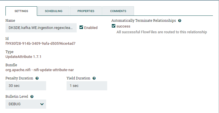
For demonstration, lets run “UpdateAttribute”processor in debug level. Then via s2s reporting tasks, fetch the Bulletin’s as Flow File, process them and send an alert via mail to the appropriate teams.

Use UpdateAttribute processor with Bulletin level of Debug to generate dummy bulletins along with the GenerateFlowFile processor as upstream connection. Make sure the Name of the processors follow an unique convention, which helps to monitor the bulletins efficiently. For example in the following UpdateAttribute processor configuration the naming convention is “<team>.<source>.<useCase>.<Purpose>.<processTask>.<Severity>”

Then, create a new site2site reporting site.

Drag and Drop an Input port from the canvas and give it a name, which should be same as the Input Port Name in the reporting tasks. Once these mundane stuffs are done, NIFI routes the bulletins to this input port.

NIFI emits the bulletins as an JSON array, So the first process is to extract the individual elements in the JSON array using SplitJson Processor.

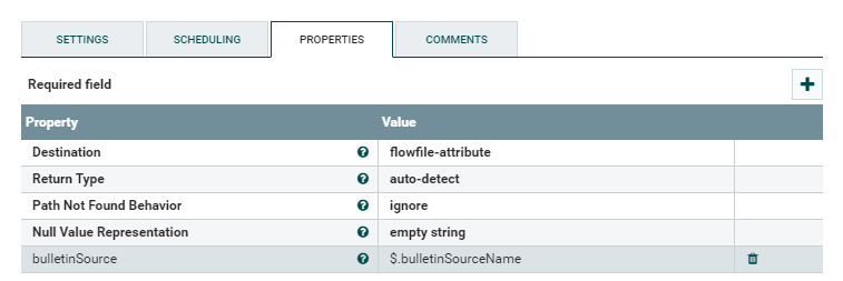
Once the individual JSON elements are splitted, extract the source name i.e. from where the bulletin is emitted, using EvaluateJsonPath processor.

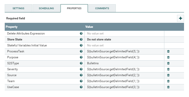
As, the bulletin source name is the actual name of the processor which we give in the format of “<team>.<source>.<useCase>.<Purpose>.<processTask>.<Severity>”.

Let’s extract the individual attribute from the source name using UpdateAttribute processor.

Use the team attribute to route for the specific processor group.

Remove duplicate bulletins to avoid bombarding with alert messages using DetectDuplicate processor.

Use the LookUpService processor to load email based on the severity levels.

If the severity level is Audit it makes sense to store it in HDFS rather than alerting via e-mail. Hence, use RouteOnAttribute to route the flow files to respective flows like PutMail processor for alerting or merge the contents and dump it in HDFS.

Conclusion

Hope, this walk-through helps you find how easy it is to monitor a NIFI data flow with the help of bulletins and built-in processors. Additionally the generated bulletins also helps in monitoring disk-usage, memory utilization and back-pressure which itself deserve separate article to cover.

This article centers around covering how to utilize compaction effectively to counter the small file problem in HDFS.

Small File Problem

HDFS is not suitable to work with small files. In HDFS a file is considered smaller, if it is significantly smaller than the HDFS default block size (I.e. 128mb).

To make HDFS faster all file names and block addresses are stored in Namenode memory. In this way, that implies, if there is any modification done in the file system or reading a file location, all of these can be served without any disk I/OS.

But this design approach to put away all metadata in memory has its own tradeoffs. One of them is that for every file, directory and block in HDFS we need to spend around 150 bytes of namenode’s memory. So, If there are millions of files, then the amount of RAM that needs to be reserved by the Namenode becomes large.

Besides, HDFS is not designed to geared up to efficiently accessing small files. It is designed to work with a small number of large files rather than working with large number of small files. Reading through small files normally causes lots of disk seeks which mitigates the performance.

Compaction to the rescue

Compaction can be used to counter small file problems by consolidating small files. This article will walk you through small file problems in Hive and how compaction can be applied on both transactional and non-transactional hive tables to overcome small files problem.

In Hive small files are normally created when any one of the accompanying scenario happen.

• Number of files in a partition will be increased as frequent updates are made on the hive table.
• Chances are high to create more number of small files (i.e. Size lesser than default HDFS block size) when the number of reducers utilized is on the higher side.
• Since there is a growing demand to query the streaming data in near real time (within 5 to 10 minutes). So the streaming data needs to be ingested into a Hive table with short interim of time, which will eventually result in lots of small files and this should be addressed in the design.

For demonstration, let’s use the following hive query to create an ‘orders’ table and then apply a compaction algorithm over it.

CREATE TABLE IF NOT EXISTS orders (id bigint,
customer_id string,
customer_name string,
product_id int,
product_name string,
product_price decimal(12,2),
quantity int,
src_update_ts timestamp,
src_file string,
ingestion_ts timestamp)
PARTITIONED BY (order_date date)
ROW FORMAT SERDE 'org.apache.hive.hcatalog.data.JsonSerDe'
LOCATION '/user/dks/datalake/orders';

The Hive table is partitioned by date and stored in the form of JSON. As this table is partitioned by date, for 5 years of data with Avg 20 files per partition, then possibly we will end up with 5* 365 * 20 = 36,500 files. Having a huge number of files may lead to performance bottlenecks.

So, let’s run a compaction algorithm out of sight periodically to combine files whenever a particular partition reaches a certain number of files, in our case it is 5.

Approach to enable compaction on Non-Transactional tables

• Find out the list of all partitions which holds more than 5 files, this can be done by using the hive virtual column ‘input__file__name’.
• Set the reducer size to define approximate file size.
• Execute insert overwrite on the partitions which exceeded file threshold count, in our case which is 5.

The hive configurations to use,

set hive.support.quoted.identifiers=none;
set hive.exec.dynamic.partition=true;
set hive.exec.dynamic.partition.mode=nonstrict;
set hive.exec.reducers.bytes.per.reducer=268435456; --256MB reducer size.

Use the accompanying hive query to perform compaction.

with partition_list as
(select order_date, count(distinct input__file__name) cnt from orders
group by order_date  having cnt > 5)
insert overwrite table orders partition (order_date)
select * from orders
where order_date  in (select order_date from partition_list)

Approach to enable compaction on Transactional tables

I have already covered about Transactional tables in one of my past articles, so please examine the same here, before proceeding further.

Given the need to apply frequent updates on the ACID enabled table, the hive can generate a large number of small files. Unlike a regular Hive table, ACID table handles compaction automatically. All it needs is some table properties to enable auto compaction.

“compactor.mapreduce.map.memory.mb” : specify compaction map job properties

“compactorthreshold.hive.compactor.delta.num.threshold: Trigger minor compaction threshold

“compactorthreshold.hive.compactor.delta.pct.threshold”: Threshold when to trigger major compaction

CREATE TABLE IF NOT EXISTS orders (id bigint,
customer_id string,
customer_name string,
product_id int,
product_name string,
product_price decimal(12,2),
quantity int,
src_update_ts timestamp,
src_file string,
ingestion_ts timestamp)PARTITIONED BY (order_date date)
CLUSTERED BY (id) INTO 10 BUCKETS STORED AS ORC
LOCATION '/user/dks/datalake/orders_acid';
TBLPROPERTIES ("transactional"="true",
"compactor.mapreduce.map.memory.mb"="3072",     -- specify compaction map job properties
"compactorthreshold.hive.compactor.delta.num.threshold"="20",  -- trigger minor compaction if there are more than 20 delta directories
"compactorthreshold.hive.compactor.delta.pct.threshold"="0.5" -- trigger major compaction if the ratio of size of delta files to          -- size of base files is greater than 50%);

Conclusion

Thus, compaction can be utilized effectively to build a robust data pipeline, which will ensure there will be of no small files.

Developing a spark application is fairly simple and straightforward, as spark provides featured pack APIs. Be that as it may, the tedious task is to deploy it on the cluster in an optimal way which yields ideal performance and following the best practices when developing spark jobs. Here in DataKareSolutions, we often need to get our hands dirty to tune the spark application. Throughout this article I will put out all the best practices we follow in DataKareSolutions to optimize spark application.

Data Serialization

Spark bolsters two types of serialization, Java serialization which is the default one and Kryo serialization. Kryo serialization is significantly faster and compact than Java serialization. Thus, in production it is always recommended to use Kryo over Java serialization. To use Kryo, the spark serializer needs to be changed to Kryo serializer in the spark configurations.

conf.set(“spark.serializer”,”org.apache.spark.serializer.KryoSerializer”)

However, Kryo may fails to serialize few classes rarely to avoid this Kryo requires you to register the classes which are expected to be serialized.

Broadcasting

If the tasks across multiple stages requires the same data, it is better to broadcast the value rather than send it to the executors with each task. And when joining two tables if one of the join is small enough to fit into memory it is advisable to broadcast it, to avoid shuffles.

Avoid UDF and UDAF

It is better to avoid UDF in favor of spark SQL functions as it avoids deserialization of data so that it can process in scala and then serialize it again. Moreover Spark SQL functions are well tested and chances are there it will yield better performance compared to UDF.

Furthermore, with regards to UDAF which produces sortAggregate which is relatively in slower side than its counterpart hashAggregates.

Data locality

To achieve better performance the data should reside as close to the computation. There are four different sorts of locality in spark.

1. PROCESS_LOCAL — Data is in the same JVM which is running the task. Obviously the best one.
2. NODE_LOCAL — Data is on the same node as the computation. Comparatively slower than process local as the data needs to travel between processes.
3. NO_PREF — No locality preference.
4. RACK_LOCAL — Data will reside on the same rack.
5. ANY — Data may reside anywhere on the network not on the same rack.

It is always preferable to choose the best locality levels to avoid data movements. But there may be times when there are no new data to process, sparks tries to fetch data from lower locality levels. Spark will wait for a certain period of time before switching to lower locality levels.

Use the accompanying parameter to configure the interval time to wait before switching locality levels.

spark.locality.wait //which is 3 seconds by default

To inspect whether a task ran locally, in the spark UI the locality_levels can be found out under stages tab.

Dynamic allocation

Spark is shipped with an excellent mechanism to use the cluster resources rather efficiently based on workloads and on shared clusters. According to the workloads it is possible to scale up and scale down the number of executors which is known as dynamic allocation.
The following configuration parameters are used to enable and tweak dynamic allocation.

spark.dynamicAllocation.enabled //Set the value to true to enable dynamic allocation.
spark.dynamicAllocation.executorIdleTimeout //Timeout to wait before releasing the executor.
Spark. dynamicAllocation. cachedExecutorIdleTimeout  //Timeout to wait before removing the cached data blocks.
spark.dynamicAllocation.initialExecutors //The initial number of executors to begin with. However, if the number of executors is explicitly mentioned via --num-executors` (or `spark.executor.instances`) then the larger value between them will be the initial executors value.
spark.dynamicAllocation.maxExecutors //Upper bound of executors, by default infinity.spark.dynamicAllocation.minExecutors //Minimum number of executors by default is '0' which ensures our application won’t occupy cluster resources unnecessarily.

When enabling dynamic allocation it is also necessary to enable Spark’s external shuffle service which can be done by the parameter spark.shuffle.service.enabled.This ensures that we have a separate server on each machine in the cluster which will manage shuffle files when the appropriate executor is removed/lost.

Garbage collection

Garbage collection can be a bottleneck in spark applications. It is advisable to try the G1GC garbage collector, which can improve the performance if garbage collection is the bottleneck. The parameter -XX:+UseG1GC is used to specify G1GC as the default garbage collector. And increase the G1GC region heap size if the executer heap size is large this can done by -XX:G1HeapRegionSize.

It is always recommended to use data structures which generated less objects, like array instead of LinkedLists.

Refer this link for in-depth explanation.

Executor Tuning

When deploying a spark application one of the most prominent thing is to allocate the execution resources optimally like number of executors, executors core and executors memory.

Number of executor cores

As the name indicated executor cores will define the number of cores to use for each executors. Each individual cores will be assigned to one different task. Therefore, we will be fancying to allocate more cores to a single executor. But too many tasks per executor will results in garbage collection overload and as a matter of fact HDFS achieves better throughput when the number of executors is set to 5.
Hence, it is always recommended to assign the number of executors cores to ~5.

As a rule of thumb one core in each node of the cluster will be allocated to OS process and Hadoop daemons.

Number of executors

Executer is just another JVM instance, so it is possible to have more than one executors.
The number of executors depends upon the number of cores in the cluster.

If the application is deployed on top of yarn, one executor will be assigned to the yarn application master.

For example, if there are 250 cores in the cluster, then the number of executors should be 250/5 = 50 executors. Out of which one should be left for application master and the remaining 49 can be assigned to our spark application by using the parameter –num-executors=49 when submitting the application for execution.

Memory per executor

As a standard guideline, one GB in each nodes of the cluster will be allocated to OS process and Hadoop daemons.

Let’s assume we have a 250 core cluster and 64 GB memory on each node. If 1 GB is allocated to Hadoop demon and OS processes, we will be left with 63 GB memory in each node.

As discussed above, we will be left with 5 executors per node if we have 25 cores per machine (i.e. 49 executors in a 250 core cluster after allocating one to yarn AM). Thus we may consider to allocate (63 GB/5 executors) = 12.6 GB to each executor.
But there is an additional yarn overhead memory needs to be allocated to each executor. The additional overhead memory is 10% by default (7% for legacy spark versions)of the executor memory. I.e. 12.6-(0.10 * 12.6)= 11.34 GB per executor is the optimal memory per executor.

Parallelism

Degree of parallelism is the most proficient parameter which dictates the performance of a spark job. The partition size should be in a form that it should not be too big which will eventually lead to under-utilization of the cluster neither too small which will lead to too much of small tasks. The partition size should be in such a way it should utilize the clusters efficiently without any overheads of small tasks.
In spark higher level APIs like dataframe and datasets use the following parameters to determine the partition of a file.

spark.sql.files.maxPartitionBytes //Specify maximum partition size by default 128mb
spark.sql.files.openCostInBytes //The approximate cost to use to open the file and scan the file which is by default 4MB.

Spark automatically figures the optimal partition size based on these two parameters.

At whatever point, if there is a shuffle operation spark will use spark.sql.shuffle.partitions parameter to determine the partition size which by default is 200 by default. It is recommended to shrink down the shuffle partitions size if the Size of the file is small.

If the dataset was derived from an RDD, it will inherit the partition size of the parent RDD.

Speculative execution

In real time use cases there are scenarios where a spark job may perform poorly compared to other worker nodes due to some external factors which may not in our control. Then spark will re-launch the same task in some other worker nodes.
Speculative execution can be enabled and can be tuned by using the accompanying parameters.

spark.speculation //Set to true to enable by default it is false.
spark.speculation.interval //Time interval to check for speculative    tasks.
spark.speculation.multiplier //specify how much times the tasks can be slower than the median to consider it as a speculative job.
spark.speculation.quantile (value in percentage) //The fraction of tasks which must be completed before speculation is enabled in a particular stage.

Spark driver will normally spend a lot of time in detecting speculation when managing a large number of tasks, enable it only if needed.

Parallel transformations

If there are multiple queries/transformations which can be executed independently it is recommended to take leverage of spark scheduler pool. By default spark executes the tasks in FIFO to execute tasks in parallel the first step is to change it into Fair, which will dictate spark to execute the job in round robin fashion. This can be done by changing the configuration parameter “spark. scheduler. mode” to FAIR in the Spark configuration object.
Then create an separate pools for different independent queries.

spark.setLocalProperty("spark.scheduler.pool", "pool1")
// Query 1
spark.setLocalProperty("spark.scheduler.pool", "pool2")
//Query 2

The most common use case for it is when writing the same streaming query
data to multiple destinations in structured streaming
Refer this link for more details.

Data Skewing

Data skewing is a condition when the data is unevenly distributed across the cluster, which causes serious performance degrades because skewed data will makes the cluster underutilized. So, if a spark job is taking more time to complete, it is always a wise decision to check for data skew. And if it proves to be true apply one of the following techniques to handle data skewing.
1. Repartition
2. Salting
3. Isolating salting
4. Isolating Map/Join
5. Iterative Broadcasting
Each of these techniques has its own advantages/limitations. Covering each of these is out of scope for this article.

Databricks delta provides some fairly simple and powerful techniques to handle Data skews.

Miscellaneous optimizations

• Throughout the spark application use only Dataframe/Dataset. Typically, there is no reason to use RDD unless you are writing your own partitioner.
• Cache Spark Sql table and dataframe. It will mimimize memory usage and Garbage collection overhead as Spark will scan only required columns and automatically tune compression.
• Avoid String for keys and consider to use numeric IDs wherever possible.

Conclusion

We have walked through the major key factors which will impact the performance of Spark jobs in detail. Go through this article which will give a good idea on how to optimize Spark joins.

If you are working in Big Data space, soon you would found yourself working with a NoSql database. HBase has a huge chunk of users and fits in most of the NoSql use cases. So, in case if you are getting started what HBase in production the following HBase commands will come in handy.

Create a employee HBase table with column families “personal” and “professonal” and follow this walkthrough.

Get by Row Key:

        get ’emp’, ‘52568’

To get row of a corresponding row key.

Row Prefix Filter

scan ’emp’, {FILTER =”(PrefixFilter(32))”}

Row Prefix Filter returns all the rows which starts with the specified row prefix in the PrefixFilter, The above HBase command will return the rows which starts with 32.

SingleColumValue Filter

scan ’emp’ { COLUMNS=>[“personal:name”,”personal:age”],FILTER =>”(SingleColumnValueFilter(‘professional’,’desig’,=,’substring:engineer’))” }

To get columns based on a value in a particular cell use SingleColumnValueFilter. The SingleColumnValueFilter needs column family, qualifier, compare operator and a comparator. The above command will return name and age from HBase column emp where the employees designation is like engineer.

Row Count for particular time range

hbase org.apache.hadoop.hbase.mapreduce.RowCounter <tablename> –starttime=[start] –endtime=[end]

HBase will launch a mapreduce job to get count the no of rows for the specified time range.

List Regions

list_regions ’emp’

List all the regions of an particular table.

Get Row Key based on pattern

scan ‘emp’, {FILTER => “RowFilter(=, ‘regexstring:^1.*’)”}

RowFilter along with regex string comparator will help to fetch the rows based on a particular regex pattern. In the above example the row Filter returns all the rows where the row key starts with 1.

Get the records in last 15 mins

cTime = System.currentTimeMillis()
sTime = System.currentTimeMillis() -15 *60*1000
scan ‘EMP’, { TIMERANGE => [sTime, cTime] }

To get the rows which are inserted in the last 15 (or any other time range) use the TimeRange filter along with the time range.

Get Specific columns based on value of any two columns

scan ’emp’ {COLUMNS=>[“personal:name”,”personal:age”],FILTER =>”(SingleColumnValueFilter(‘professional’,’desig’,=,’substring:engineer’) AND SingleColumnValueFilter(‘professional’,’exp’,=,’binary:5′))”}

Combine filters to filter out the specific records. This query will return name and age columns from HBase table emp where the designation is like engineer and experience is 5 years.

Joins

There may arise a scenario that one may need to join two HBase tables. The best solution in this case is to create an Table in Hive or Impala over the HBase tables and perform the joins on Hive/Impala tables.

Please refer this link for HBase – Hive Integration

This article is a continuation of my previous article, which you can peruse here. Like the previous one this article also walks you through all the three sorts of Incremental Ingestion which should be possible on Hive tables yet just this time the tables are ACID enabled.

For demonstration purpose, we will be using the same example from the previous article. Let’s Start with creating a stage table for the same ‘orders’ data.

Step 1: Create Hive Stage Table

CREATE EXTERNAL TABLE IF NOT EXISTS orders_stg (id string,
customer_id string,
customer_name string,
product_id string,
product_name string,
product_price string,
quantity string,
order_date string,
src_update_ts string)
ROW FORMAT SERDE 'org.apache.hive.hcatalog.data.JsonSerDe'
LOCATION '/user/dks/datalake/orders_stg';
/user/dks/datalake/orders_stg  // Location of the source data

Step 2: ACID enabled Tables in Hive

As to keep up with the consistency of database before and after transactions, certain properties are followed. ACID stands for four traits of database transactions which are,

Atomicity: A task either succeeds totally or fizzles, it doesn’t leave halfway information.

Consistency: Once an application performs an operation the results of that operations are notified to it in each subsequent activity.

Isolation: Anincomplete operation by one user/client does not cause startling reactions for different users/clients.

Durability: when an operation is finished it will be preserved even withstanding machine or system failure.

These qualities have for some time been anticipated from database systems as part of their transaction functionality.

ACID transaction table functionality is available from Hive version 0.13.

The principle motivation behind introducing ACID tables in Hive is to address following situations:

1. Streaming Data Ingestion to Hive tables with frequent updates and insert data, enabling readers to get consistent view of data.
2. To counter too many small files.
3. Slowing changing functionality to Hive table.
4. Bulk Updates using SQL Merge.

Please note that ACID tables still doesn’t bolster commit and rollback. Only ORC file format is supported. Tables must be bucketed in order to utilize this feature.

In an “ACID” enabled table, data is stored as a set of base files. New records, updates, and deletes are stored as delta files. For each transactions a new set of delta files are created.When reading the data from table, the reader blends the base and delta records, applying any updates and deletes as it reads.

Having so many delta/small files can lead to performance issues, this can be addressed by utilizing the compaction process which combines the delta files. Compaction is explained in the later part of this subject.

Defining Acid enabled Tables

To define an ACID enabled table in Hive use the accompanying configuration parameters,

Set hive.enforce.bucketing=true
Set hive.exec.dynamic.partition.mode= nonstrict
Set hive.support.concurrency=true

and set the “transactional”=”true” table property on HIVE DDL query which enables the ACID features on Hive table.

CREATE TABLE IF NOT EXISTS orders (id bigint,
customer_id string,
customer_name string,
product_id int,
product_name string,
product_price decimal(12,2),
quantity int,
src_update_ts timestamp,
src_file string,
ingestion_ts timestamp)
PARTITIONED BY (order_date date)
CLUSTERED BY (id) INTO 10 BUCKETS STORED AS ORC
LOCATION '/user/dks/datalake/orders_acid';
TBLPROPERTIES ("transactional"="true")

Step 3: Ingestion

The following query can be used to perform insert/update or delete based on the requirements.

with new_data_stg as  (select * from orders_stg)
MERGE INTO orders AS T
USING new_data_stg AS S
ON T.ID = S.ID and T.order_date = S.order_date
WHEN MATCHED AND (T.quantity != S.quantity AND S.quantity IS NOT NULL) THEN UPDATE SET quantity = S.quantity, src_update_ts = S.src_update_ts
WHEN MATCHED AND S.quantity IS NULL THEN DELETE
WHEN NOT MATCHED THEN INSERT VALUES (S.ID, S.customer_id, s.customer_name, s.product_id, s.product_name, s.product_price,quantity,src_update_ts,ingestion_ts, cast
(order_date as date));

As mentioned above the disadvantage with this approach is each time an update/insert or delete operation is performed on a partition or table, Hive creates delta files which results in huge number of small delta files. Which can hinder the performance while reading the data. To counter this, enable auto compactor option on the table so that Hive can perform major and minor compaction out of sight to combine small/delta files.

The revised query to enable compaction on the hive table:

CREATE TABLE IF NOT EXISTS orders (id bigint,
customer_id string,
customer_name string,
product_id int,
product_name string,
product_price decimal(12,2),
quantity int,
src_update_ts timestamp,
src_file string,
ingestion_ts timestamp)
PARTITIONED BY (order_date date)
CLUSTERED BY (id) INTO 10 BUCKETS STORED AS ORC
LOCATION '/user/dks/datalake/orders_acid';
TBLPROPERTIES ("transactional"="true",
"compactor.mapreduce.map.memory.mb"="3072",     -- specify compaction map job properties
"compactorthreshold.hive.compactor.delta.num.threshold"="20",  -- trigger minor compaction if there are more than 20 delta directories
"compactorthreshold.hive.compactor.delta.pct.threshold"="0.5" -- trigger major compaction if the ratio of size of delta files to          -- size of base files is greater than 50%
);

Conclusion

So far we have covered various sorts of methods to perform incremental ingestion on Hive table and ACID enabled hive tables. As discussed, based on the criteria and requirement choose the suitable ingestion type.

Please feel free to contact me at my twitter account, if you have any sort of queries.

Joins are one of the fundamental operation when developing a spark job. So, it is worth knowing about the optimizations before working with joins.
In Data Kare Solutions we often found ourselves in situations to joining two big tables (data frames) when dealing with Spark SQL. In this article we put out the best practices and optimization techniques we used to pursue when managing Spark Joins.

Spark approaches two types of cluster communication Strategy:

• node-node communication strategy
• per-node communication strategy

In node-node communication Spark shuffles the data across the clusters, whereas in per-node strategy spark perform broadcast joins.

Performance of Spark joins depends upon the strategy used to tackle each scenario which in turn relies on the size of the tables. Sort Merge join and Shuffle Hash join are the two major power horses which drive the Spark SQL joins. Despite the fact that Broadcast joins are the most preferable and efficient one because it is based on per-node communication strategy which avoids shuffles but it’s applicable only for a smaller set of data. Thus, more often than not Spark SQL will go with both of Sort Merge join or Shuffle Hash.

Sort -Merge Join

Sort-Merge join is composed of 2 steps. The first step is to sort the datasets and the second operation is to merge the sorted data in the partition by iterating over the elements and according to the join key join the rows having the same value.

From spark 2.3 Merge-Sort join is the default join algorithm in spark. However, this can be turned down by using the internal parameter ‘spark.sql.join.preferSortMergeJoin’ which by default is true.

To accomplish ideal performance in Sort Merge Join:
• Make sure the partitions have been co-located. Otherwise, there will be shuffle operations to co-locate the data as it has a pre-requirement that all rows having the same value for the join key should be stored in the same partition.
• The DataFrame should be distributed uniformly on the joining columns.
• To leverage parallelism the DataFrame should have an adequate number of unique keys

Broadcast joins

Easily Broadcast joins are the one which yield the maximum performance in spark. However, it is relevant only for little datasets. In broadcast join, the smaller table will be broadcasted to all worker nodes. Thus, when working with one large table and another smaller table always makes sure to broadcast the smaller table. We can hint spark to broadcast a table.

import org.apache.spark.sql.functions.broadcast
val dataframe = largedataframe.join(broadcast(smalldataframe), "key")

Recently Spark has increased the maximum size for the broadcast table from 2GB to 8GB. Thus, it is not possible to broadcast tables which are greater than 8GB.

Spark also internally maintains a threshold of the table size to automatically apply broadcast joins. The threshold can be configured using “spark.sql.autoBroadcastJoinThreshold” which is by default 10mb.
So, it is wise to leverage Broadcast Joins whenever possible and Broadcast joins also solves uneven sharding and limited parallelism problems if the data frame is small enough to fit into the memory.

Shuffle Hash Join

Shuffle Hash join works based on the concept of map reduce. Map through the data frames and use the values of the join column as output key. Shuffles the data frames based on the output keys and join the data frames in the reduce phase as the rows from the different data frame with the same keys will ended up in the same machine.

Spark chooses Shuffle Hash join when Sort merge join is turned off or if the key is not suitable and also based on the accompanying two functions.

def canBuildLocalHashMap(plan:LogicalPlan):Boolean= { plan.statistics.sizeInBytes < conf.autoBroadcastJoinThreshold * conf.numShufflePartitions
}

As the name of the function indicates Spark uses this function to make sure Shuffle Hash join is better suitable for the given dataset than broadcast join. But, there might be a few situations where some scenarios join will be superior to anything Shuffle Hash join.

So, at that point we may increase the automatic broadcast join threshold size (‘spark.sql.autoBroadcastJoinThreshold’) to trick the catalyst optimizer to use Broadcast join.

def muchSmaller(a: LogicalPlan, b: LogicalPlan): Boolean = { a.statistics.sizeInBytes * 3 <= b.statistics.sizeInBytes
}

Creating hash tables are costly and it can be only done when the average size of a single partition is small enough to build a hash table.

Sort merge join is a very good candidate in most of times as it can spill the data to the disk and doesn’t need to hold the data in memory like its counterpart Shuffle Hash join. However, when the build size is smaller than the stream size Shuffle Hash join will outperform Sort Merge join.

The factors which decide the performance in the Shuffle Hash Join is same as the one in the Sort Merge Join, except it doesn’t necessarily need the partitions should be co-located.

• The DataFrame should be distributed evenly on the joining columns.
• To leverage parallelism the DataFrame should have an adequate number of unique keys.

Tips: During joins if there are rows which are irrelevant to the key, filter the rows before the join. Otherwise, there will be more data shuffle over the network.

Conclusion

Thus we have walked through the different types of algorithms used by spark for joins. Try to use Broadcast joins wherever possible and filter out the irrelevant rows to the join key to avoid unnecessary data shuffling.

And for cases if you are confident enough that Shuffle Hash join is better than Sort Merge join, disable Sort Merge join for those scenarios.